Principal Component Analysis (PCA)

Overview

Principal Component Analysis (PCA) is a dimensionality reduction technique that transforms high-dimensional data into a smaller set of uncorrelated features, called principal components, while preserving as much variance as possible. It works by identifying directions (components) that capture the most variation in the dataset, ranking them based on their importance. The first few components usually contain the majority of the information, allowing for data visualization, noise reduction, and improved model performance.

In this project, PCA was applied to transform the dataset into a lower-dimensional space, making it easier to analyze while preserving 95% of the variance. The process involved standardizing the data, computing principal components, and selecting the optimal number of components for effective modeling.

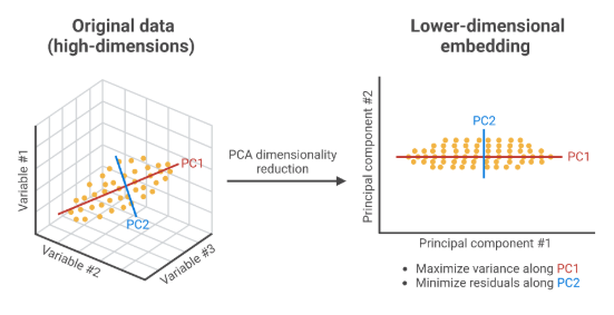
The image above shows how PCA (Principal Component Analysis) helps reduce high-dimensional data into a simpler, lower-dimensional form. On the left, data with three variables is shown in 3D. PCA finds new directions, called principal components, that capture the most variation in the data. The right side shows how the data is projected onto just two components (PC1 and PC2), keeping most of the important information while making it easier to work with and visualize.

Although PCA is a powerful technique, it can make transformed features harder to interpret as they no longer align with original variable meanings. However, it remains an effective tool for improving model performance, speeding up computations, and gaining insights through visualization.

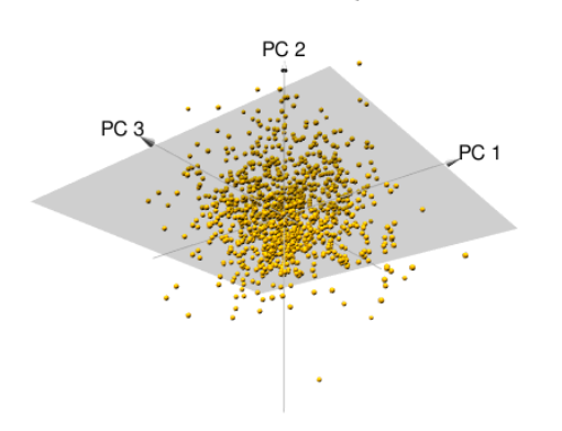
This image visualizes the result of applying PCA on a dataset with three dimensions. The yellow dots represent data points in 3D space, and the gray plane shows the lower-dimensional space formed by the first two principal components, PC1 and PC2. PCA projects the data onto this plane because it captures the majority of the data’s variance. PC3, which contributes less to the overall variance, is not used in the projection. This helps simplify the data while still preserving the most important patterns for analysis or modeling.

Orthogonality is a key concept in PCA because it ensures that each principal component captures unique, non-overlapping information from the dataset. Since the components are orthogonal, they are uncorrelated, meaning no redundancy exists between them. This helps in breaking down complex data into clean, independent directions of variation, making the analysis more interpretable and reducing noise. Orthogonality also ensures that each component adds distinct value to the transformed dataset, improving both visualization and the performance of downstream machine learning models.

Data Selection and Preprocessing

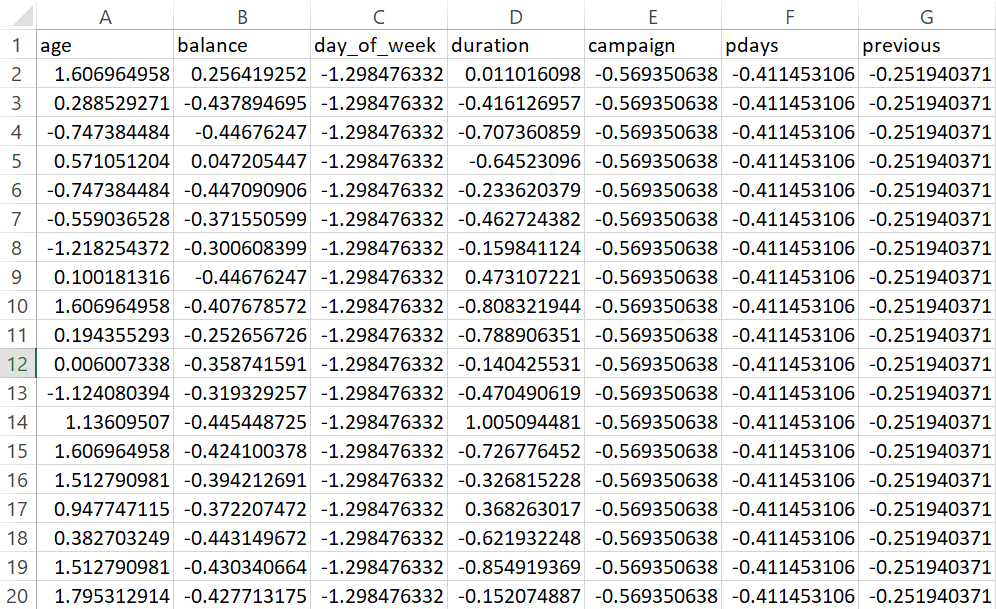
To ensure that all numerical features contribute equally to the PCA process, the dataset was standardized using StandardScaler from sklearn. Standardization transforms the data so that each feature has:

• Mean = 0
• Standard Deviation = 1

This prevents features with larger numerical ranges (e.g., balance or duration) from dominating those with smaller ranges. Only numerical columns were selected for PCA, and the standardized dataset was prepared for dimensionality reduction.

Why StandardScaler?

StandardScaler is used to normalize the dataset before applying PCA to ensure that all features contribute equally. Without standardization, features with larger numerical ranges (e.g., balance, duration) would dominate those with smaller ranges, distorting the principal components.

StandardScaler transforms the data by centering it around zero (mean = 0) and scaling it to unit variance (standard deviation = 1). This step is crucial for PCA, as it relies on variance to determine the importance of each principal component.

Applying PCA with 2 and 3 Components

To visualize and analyze the dataset in a lower-dimensional space, PCA was performed with 2 and 3 components:

Variance Retention in PCA

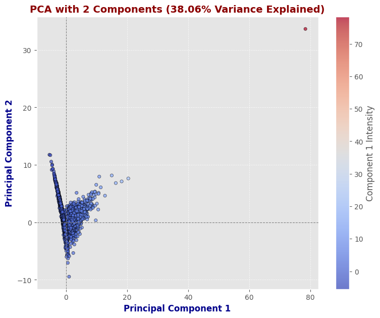
• PCA with 2 components retains 38.06% of the variance, meaning that this lower-dimensional representation captures only part of the dataset’s structure, losing a significant amount of information.
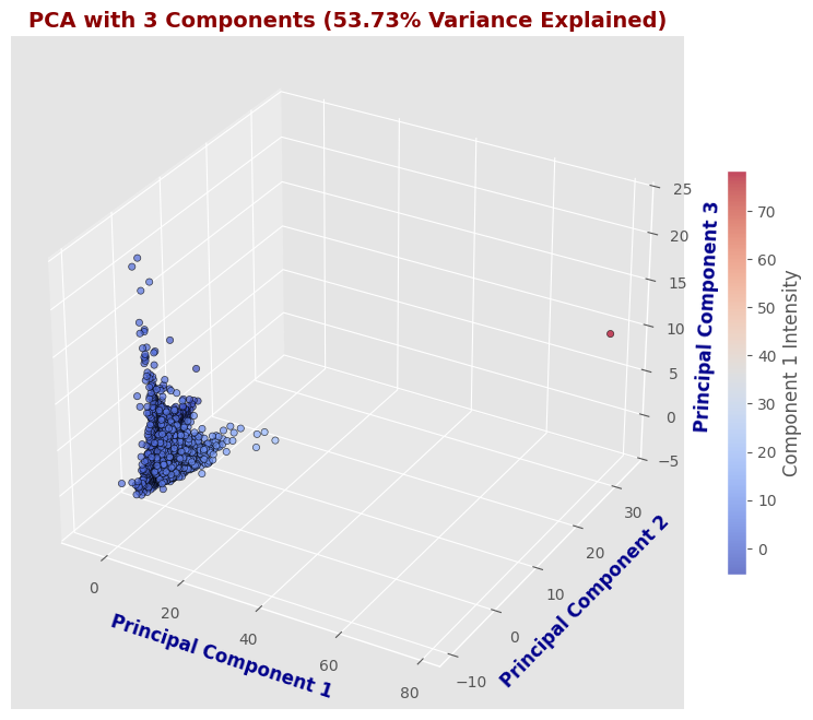
• PCA with 3 components retains 53.73% of the variance, providing a more detailed representation but still missing nearly half of the original variance.

PCA Code and Output

# perform PCA with 2 and 3 components
pca_2 = PCA(n_components=2)
pca_3 = PCA(n_components=3)

df_pca_2 = pca_2.fit_transform(df_scaled)
df_pca_3 = pca_3.fit_transform(df_scaled)

# explained variance ratio
explained_variance_2 = np.sum(pca_2.explained_variance_ratio_) * 100
explained_variance_3 = np.sum(pca_3.explained_variance_ratio_) * 100

# explained variance percentages
explained_variance_2, explained_variance_3
  

These values indicate that while PCA reduces complexity, using only 2 or 3 components is insufficient to fully preserve the dataset's structure. The corresponding cumulative variance plots shown below visually confirm the variance retained at each component level.

PCA with 2 Components

This scatter plot represents the dataset after applying PCA with 2 components, capturing 38.06% of the total variance. Most data points are clustered near the origin, with a few outliers. While this reduction helps in visualization, it does not retain enough variance for accurate modeling.

PCA with 3 Components

The 3D scatter plot provides a more informative representation by adding a third principal component, retaining 53.73% of the variance. While this visualization offers better data separation than the 2D version, it still does not preserve the majority of the dataset’s information.

Determining the Optimal Number of PCA Components

The code below performs PCA on the entire dataset to determine the number of principal components needed to retain at least 95% of the variance. By computing the cumulative explained variance, it was found that 7 principal components are required to achieve this threshold. Additionally, the top three eigenvalues were extracted (1.5093, 1.1550, and 1.0970), indicating the relative importance of the first three principal components in capturing variance. This confirms that while dimensionality reduction is effective, retaining too few components would lead to significant information loss.

# perform PCA with all components to find the number needed for 95% variance
pca_full = PCA()
pca_full.fit(df_scaled)

# cumulative explained variance
cumulative_variance = np.cumsum(pca_full.explained_variance_ratio_)

# find the number of components needed for 95% variance
num_components_95 = np.where(cumulative_variance >= 0.95)[0][0] + 1

# extract the top 3 eigenvalues
top_3_eigenvalues = pca_full.explained_variance_[:3]

num_components_95, top_3_eigenvalues
  

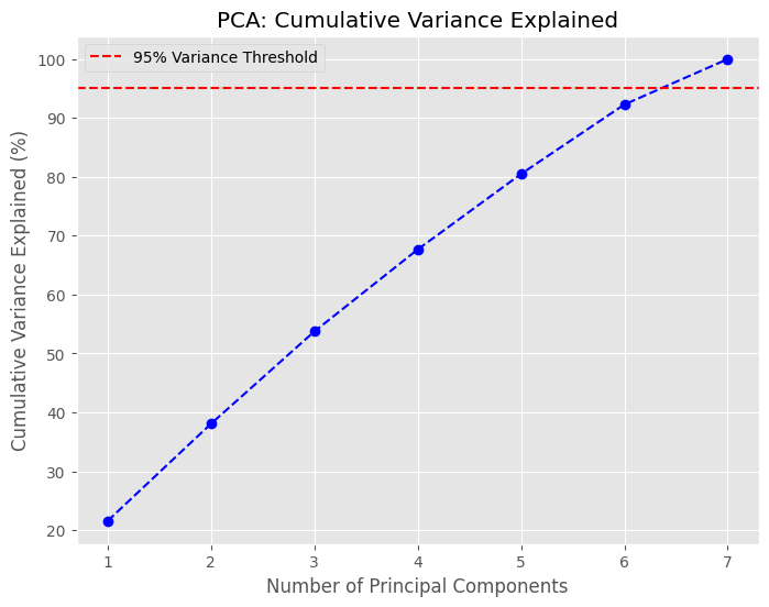
Cumulative Variance Explained by PCA Components

The graph illustrates how the cumulative variance increases as more principal components are added. The red dashed line marks the 95% variance threshold, which is reached at 7 principal components. This means that reducing the dataset to 7 dimensions preserves most of the original information while significantly lowering complexity. The plot confirms that using fewer components (e.g., 2 or 3) retains only a fraction of the variance, leading to potential information loss.

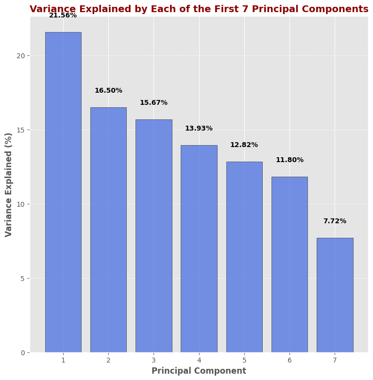
Illustration of the 7 Principal Components

This bar plot shows the variance explained by each of the first 7 principal components. The first principal component contributes the most variance (21.56%), followed by the second (16.50%) and third (15.67%). The variance contribution gradually decreases with each additional component.

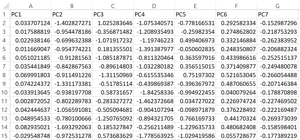
The PCA-transformed dataset represents the original features in a reduced-dimensional space, capturing 95% of the variance with 7 principal components (PC1 to PC7). Each principal component is a linear combination of the original features, optimized to retain the most critical information while reducing complexity. This transformation enables efficient modeling and visualization while minimizing information loss.

Conclusion

The PCA analysis successfully reduced the dataset’s dimensionality while preserving key information. The 2D and 3D projections revealed underlying data patterns, making it easier to identify trends and relationships.

• The 2D PCA projection retained 38.06% of the variance, providing a simplified yet informative representation of the data.
• The 3D PCA projection captured 53.73% of the variance, offering a more detailed but still reduced view of the dataset.

Further analysis showed that 7 principal components were needed to retain at least 95% of the variance, ensuring minimal information loss.

The most important principal components were those associated with key financial and engagement attributes, highlighting their influence on customer behavior. Overall, PCA played a crucial role in reducing complexity, improving visualization, and enhancing further analyses like clustering while retaining the dataset’s most significant characteristics.