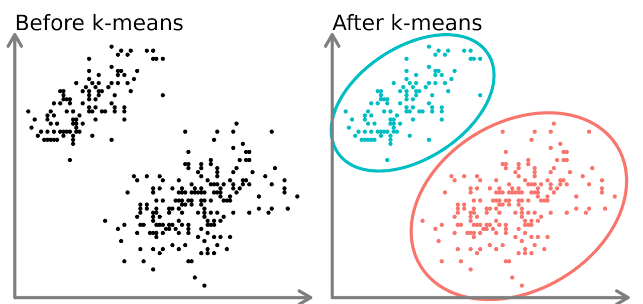
Clustering is an unsupervised learning technique that groups data points based on their similarity. It is used to identify patterns and segment data without predefined labels. The goal is to minimize intra-cluster distance (points within a cluster should be close together) and maximize inter-cluster distance (different clusters should be well-separated).
In this project, clustering was applied to segment customers based on financial and behavioral attributes, helping optimize marketing strategies and customer engagement. Different clustering techniques were explored to compare their effectiveness in revealing meaningful groupings.
Distance Metrics in Clustering
Distance metrics determine how similar or different two data points are. The most common ones include:
1. Euclidean Distance
d(i, j) = √(Σ(xᵢ − xⱼ)²)
Best for: K-Means, DBSCAN, Hierarchical Clustering (single linkage).
Measures straight-line distance between points.
Ideal for low-dimensional spaces.
2. Manhattan Distance (L1 Norm)
d₁(I₁, I₂) = Σ |I₁ᵖ − I₂ᵖ|
Best for: Grid-based clustering.
Uses sum of absolute differences.
Suitable for city-block-like data.
3. Cosine Similarity (Angle-Based)
cos(θ) = (A · B) / (‖A‖‖B‖) = Σ AᵢBᵢ / √(Σ Aᵢ² · Σ Bᵢ²)
Best for: High-dimensional data (e.g., text data, document clustering).
Measures angle between two vectors, not magnitude.
Useful when direction matters more than distance.
4. Mahalanobis Distance
D² = (x − m)T · C−1 · (x − m)
Best for: Data with correlated features or different scales.
Accounts for variance and correlation structure.
Useful in multivariate anomaly detection and clustering.
Comparison of Clustering Techniques
The three main clustering methods, K-Means,
Hierarchical Clustering, and
DBSCAN, each have unique approaches to identifying patterns within the data.
K-Means Clustering (Partition-Based)
Divides data into k predefined clusters by minimizing the distance between data points and cluster centroids.
Requires selecting the number of clusters (k) in advance.
Works well for globular, well-separated clusters but struggles with complex shapes and noise.
Distance Metric Used: Euclidean Distance.
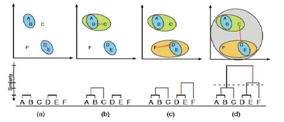
Hierarchical Clustering
Builds a tree-like structure (dendrogram) by iteratively merging or splitting clusters.
Does not require specifying k beforehand but requires a cut-off point to determine final clusters.
More computationally expensive but useful for discovering hierarchical relationships in data.
Distance Metrics Used:
Single Linkage → Uses minimum Euclidean distance.
Complete Linkage → Uses maximum Euclidean distance.
Ward’s Method → Uses Mahalanobis distance to minimize variance.
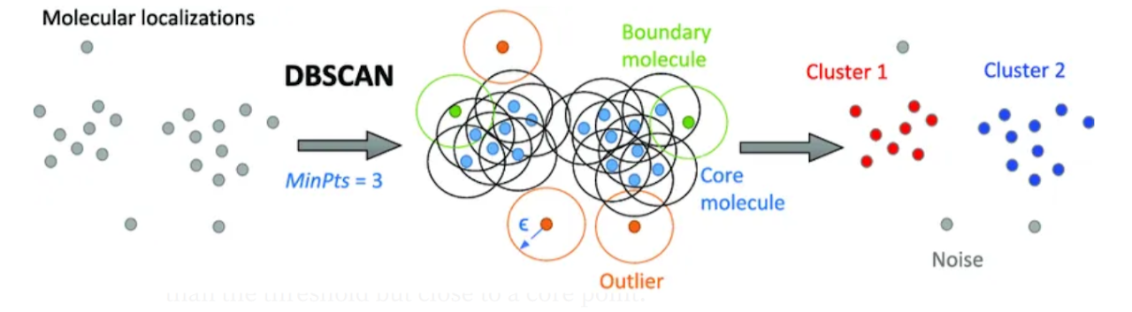
DBSCAN (Density-Based Clustering)
Groups points based on density rather than distance, identifying clusters of varying shapes and sizes.
Can detect outliers as noise, unlike K-Means and Hierarchical Clustering.
Works well for arbitrarily shaped clusters but struggles with varying densities and parameter tuning.
Choosing the right distance metric is critical in clustering because it impacts:
The shape of clusters: Euclidean distance works best for spherical clusters, while Mahalanobis accounts for correlations in the data.
The interpretability of results: Cosine similarity is ideal for text-based or high-dimensional clustering, where direction matters more than magnitude.
Scalability: Manhattan distance can be computationally cheaper and more efficient in some scenarios compared to Euclidean.
In this project, K-Means, Hierarchical Clustering, and DBSCAN were tested using Euclidean distance to identify the best segmentation strategy for customer data. The results showed that K-Means with k=2 provided the most effective clustering, while DBSCAN helped highlight potential outliers.
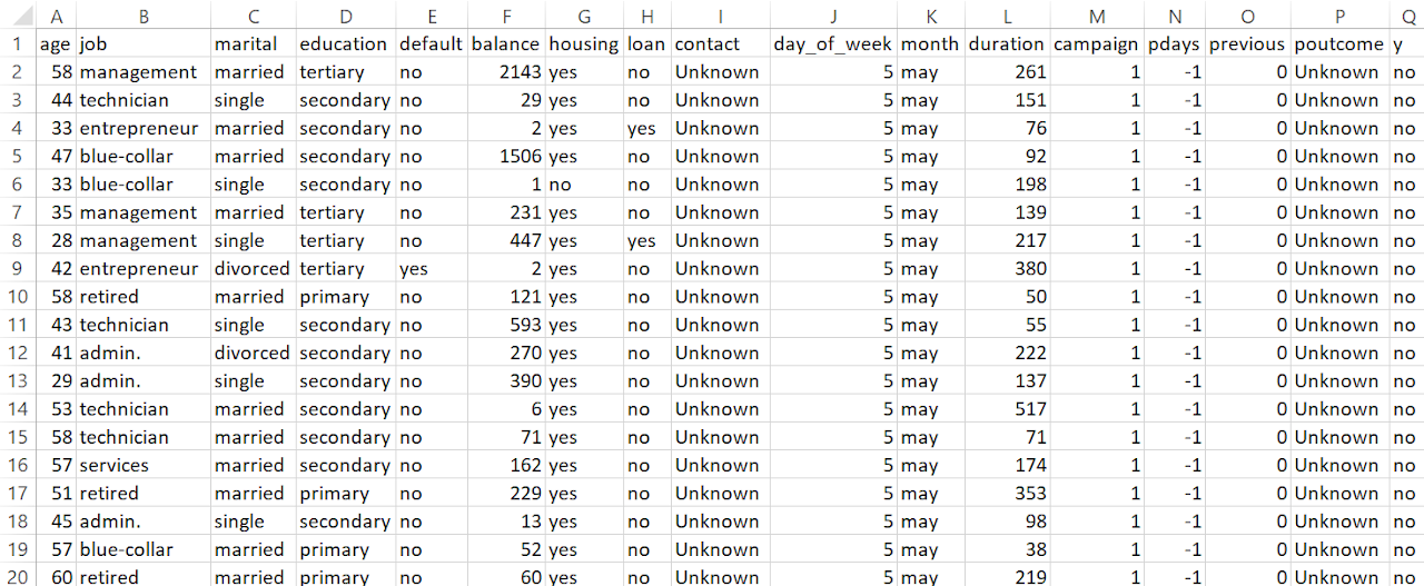
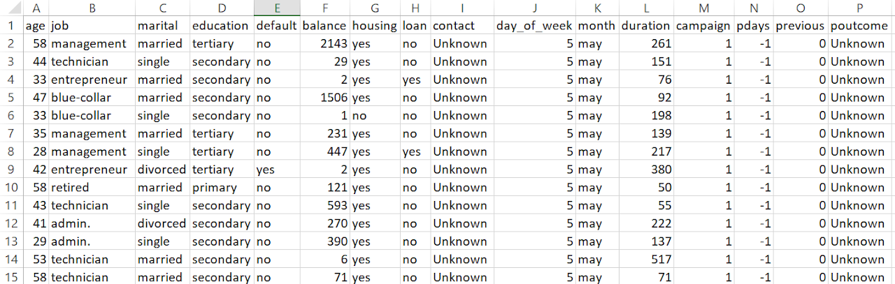
Before applying clustering algorithms, the dataset underwent careful preprocessing. Categorical variables were converted using one-hot encoding, and numerical variables were standardized to ensure fair distance measurements. Irrelevant or redundant features were removed to improve clustering performance.
The dataset was preprocessed for clustering by removing the target variable (y). This label was stored separately to evaluate clustering results post-analysis. By excluding the output label during clustering, the unsupervised nature of the algorithm is preserved, allowing natural groupings to emerge from the input features alone.
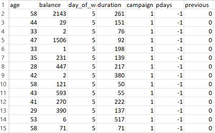
To prepare the data for clustering, only numerical columns were retained. Clustering algorithms like K-Means and DBSCAN rely on distance metrics, which require numerical input to compute meaningful similarities between data points. Removing categorical features ensures more consistent and interpretable clustering results.
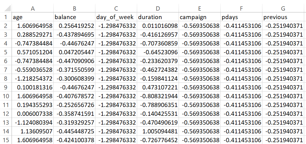
All numerical features were standardized using StandardScaler. This transformation ensures each feature has a mean of 0 and standard deviation of 1, eliminating bias caused by different feature scales. Standardization is essential for clustering techniques that use distance-based metrics.
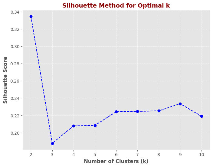
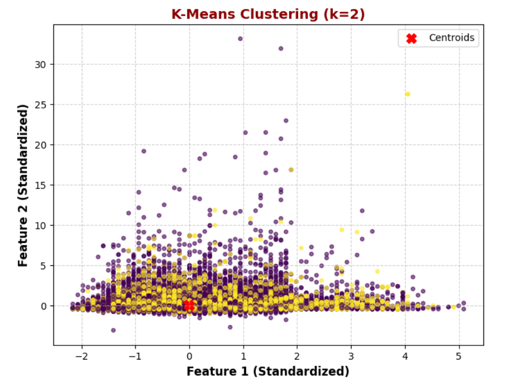
K-Means clustering was performed to segment the dataset, with k = 2 identified as the optimal number of clusters based on the Silhouette Score. The clustering results demonstrate two well-separated groups, preventing over-segmentation and maintaining interpretability. Compared to higher k values, k = 2 provides the best balance between simplicity and accuracy, making it the preferred choice for clustering.
Silhouette score plot showing k = 2 as the optimal number of clusters
The Silhouette Score plot suggests that k = 2 is the optimal choice for clustering, as it has the highest silhouette score (~0.34). This indicates that the dataset is best separated into two well-defined clusters with minimal overlap. While other values such as k = 6 and k = 9 also show moderate scores, their separation is weaker compared to k = 2. Choosing k = 2 ensures that the clusters are more distinct and compact, making it the most effective option for K-Means clustering in this scenario.
K-Means Cluster Comparison
K = 2: Well-separated clusters, most optimal
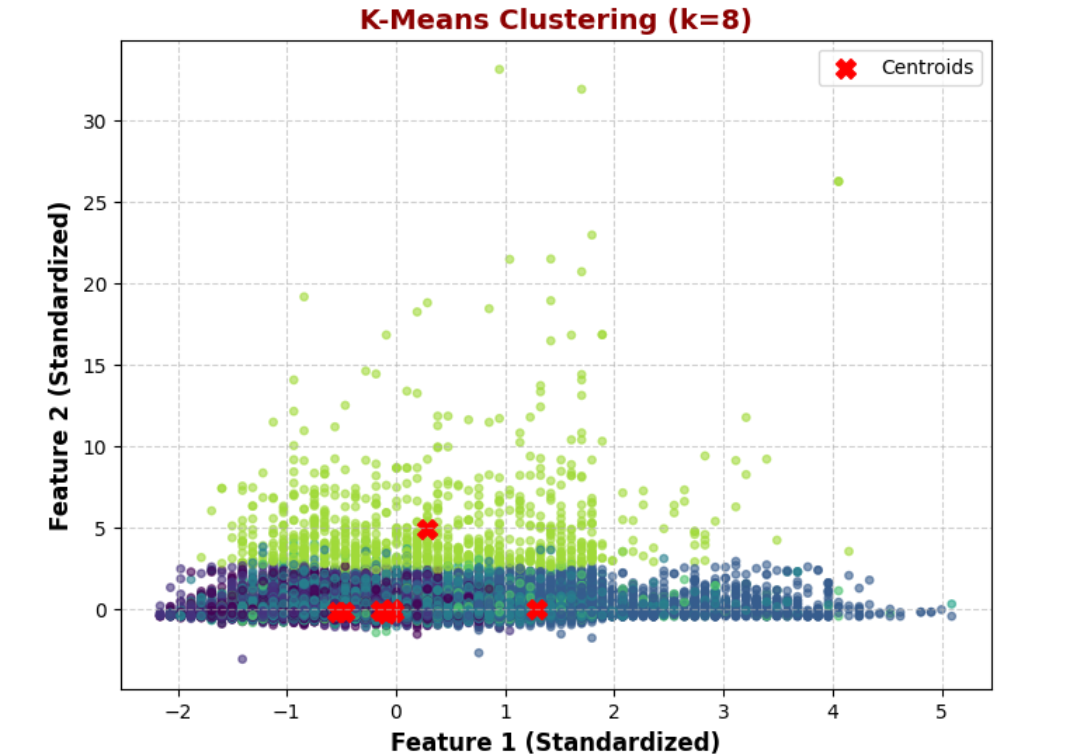
K = 8: Over-segmentation, less interpretability
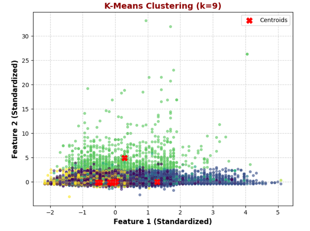
K = 9: Similar to k=8, less compact clusters
K-Means Clustering Analysis
1. K-Means with k = 2
The dataset is split into two broad groups.
The clusters show some overlap, suggesting a binary split may not fully capture complexity.
Silhouette Score indicates k=2 is optimal, though potential subclusters exist.
2. K-Means with k = 9
More distinct groups are formed, capturing finer data variations.
Some clusters are closely packed, risking overfitting with unnecessary complexity.
Centroids are well-spread, aiming for balanced group division.
3. K-Means with k = 8
Similar structure to k=9 but with slightly larger clusters.
Some clusters appear redundant or overlapping.
Higher k may reduce interpretability due to dense overlaps.
Why k = 2 is the Best Choice?
Most Distinct Separation: Simplifies the data into two broad groups.
Insights do not improve significantly—added complexity with minimal gain.
Conclusion: K=2 offers the best balance of clarity and statistical strength. It aligns with the silhouette analysis and provides a practical segmentation of the customer data.
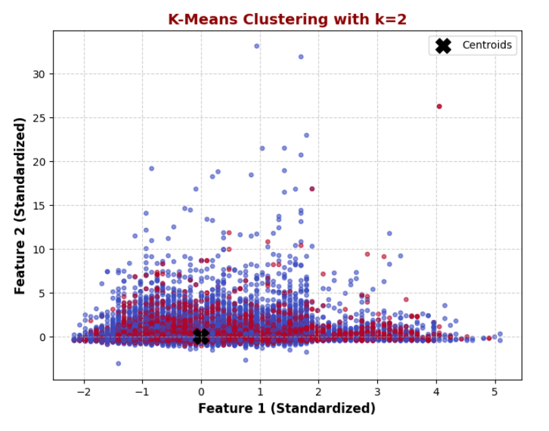
CONCLUSION: K-Means Clustering (k = 2)
The K-Means clustering (k=2) effectively divided the dataset into two distinct groups, revealing natural patterns within the data. The centroids (black markers) represent the center of each cluster, showing the average characteristics of each group. The visualization highlights a clear segmentation, indicating that the dataset has inherent structure that can be leveraged for strategic decision-making. The overlap in some areas suggests that while the clusters are distinct, there may be some similarity between certain data points.
This segmentation provides valuable insights for customer profiling and targeted marketing. If one cluster represents high-engagement customers, personalized campaigns can be tailored to maximize conversion rates. Meanwhile, the other cluster might indicate low-engagement customers, requiring different outreach strategies. This analysis confirms that K-Means is an effective technique for understanding customer behavior, enabling businesses to optimize resource allocation and enhance decision-making.
HIERARCHICAL CLUSTERING
Two distance metrics were explored:
Euclidean Distance (Ward’s Method): Groups points based on magnitude while minimizing intra-cluster variance.
Cosine Distance: Clusters points based on the angle between vectors, focusing on pattern similarity rather than size. This provides a different perspective on the data, often useful when dealing with high-dimensional or behaviorally similar data.
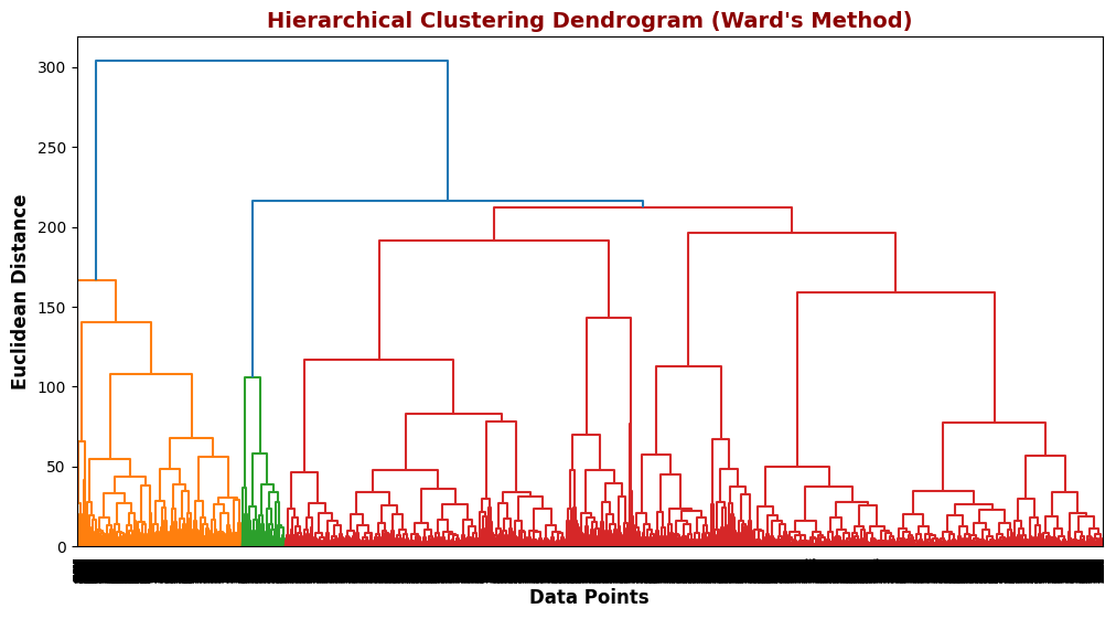
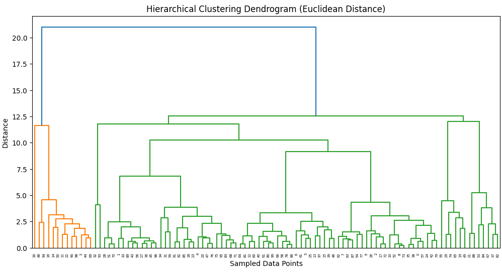
Dendrogram Using Euclidean Distance
Hierarchical clustering was applied using Ward's method, which minimizes variance within clusters. The dendrogram visualization helps determine the optimal number of clusters by identifying natural splits in the data. The structure suggests hat two main clusters can be formed, aligning with the K-Means results. Compared to K-Means, hierarchical clustering provides a more interpretable, tree-like structure, making it useful for understanding relationships between data points.
The Hierarchical Clustering Dendrogram, generated using Ward’s method, illustrates how data points are hierarchically merged into clusters. The clear separation at higher distances suggests that two main clusters naturally emerge, reinforcing findings from K-Means clustering. Unlike K-Means, this method does not require a predefined number of clusters, making it valuable for exploratory analysis and understanding the dataset's structure.
The dendrogram represents how data points are iteratively merged into clusters based on their similarity. The y-axis (Euclidean Distance) shows the linkage distance at which clusters are combined.
To avoid an overcrowded and unreadable dendrogram, a random subset of 100 data points was selected from the full dataset. This allows for clearer visualization of the hierarchical clustering structure without compromising interpretability. Sampling ensures that the dendrogram remains meaningful and visually clean while still capturing the general clustering patterns in the data.
Key Observations
Two main clusters emerge:
The large vertical jumps in the dendrogram suggest that splitting the data at this level would result in two distinct groups. This aligns with the K-Means (k=2) results, reinforcing that the dataset naturally separates into two main clusters.
Shorter branches at the bottom:
Represent data points that are very similar and were merged earlier in the process.
Larger vertical distances between merges:
Indicate less similar groups being combined, meaning the dataset has some structure but is not highly segmented.
Sampling 100 points:
Helped simplify the plot and made the cluster structure easier to interpret.
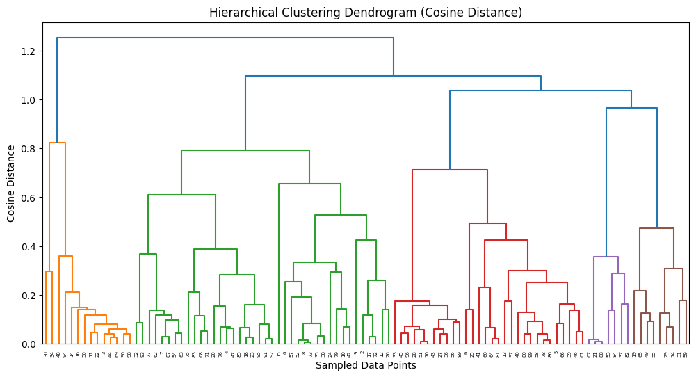
Dendrogram Using Cosine Distance
The dendrogram above illustrates the results of hierarchical clustering using
cosine distance as the similarity measure and
average linkage as the clustering method.
Unlike Euclidean distance, which considers the absolute difference between points,
cosine distance measures the angle between vectors, focusing on their direction rather than magnitude.
This is particularly useful when working with high-dimensional or normalized data,
where the pattern of attributes
matters more than their actual values.
Key Observations
The y-axis represents cosine distance,
ranging from 0 (perfect similarity)
to 1 (complete dissimilarity),
with cluster merges shown as vertical lines.
Several clusters form at low cosine distances,
indicating tightly grouped, directionally similar data points.
Higher in the dendrogram, a significant merge
occurs, suggesting a natural split between two major clusters,
similar to the result from the Euclidean-based dendrogram and K-Means with k = 2.
The structure indicates that cosine similarity
captures meaningful relationships in the data,
validating clustering results from a different perspective.
Why Use Cosine Distance?
It is scale-invariant: clustering is based on vector orientation rather than length.
Ideal for sparse or behavioral datasets (e.g., text, customer interactions) where the shape of data matters more than size.
Offers a complementary view to Euclidean-based clustering, strengthening the interpretability of results.
Comparison of Dendrogram (Hierarchical Clustering) vs. K-Means Results
Similar Findings: k=2 is the Best Choice
The dendrogram suggests two natural clusters, as seen in the large vertical jump in the hierarchy.
This supports the K-Means result where k=2 was found to have the highest Silhouette Score, indicating well-separated clusters.
Both methods agree that the dataset is best segmented into two main groups.
Key Takeaways
Hierarchical Clustering confirms the K-Means result that the data naturally separates into two clusters.
K-Means is computationally faster, making it better for large datasets.
Hierarchical Clustering provides better interpretability, allowing a flexible choice of clusters without needing to predefine k.
If cluster relationships are important, the dendrogram is more useful, as it shows how clusters are formed step by step.
CONCLUSION: Hierarchical Clustering
In conclusion, both K-Means and Hierarchical Clustering consistently revealed that the dataset naturally separates into two distinct clusters. The use of Euclidean and cosine distances in hierarchical clustering provided complementary perspectives, magnitude-based and pattern-based similarity, strengthening the reliability of the findings. Truncating the dendrogram by sampling data improved visualization without compromising insight. While K-Means offers speed and scalability, hierarchical clustering adds interpretability and flexibility, making the combined approach a robust strategy for uncovering the dataset’s underlying structure.
DBSCAN
What is DBSCAN?
DBSCAN (Density-Based Spatial Clustering of Applications with Noise) is an unsupervised machine learning algorithm designed to identify clusters based on data density. Unlike K-Means, DBSCAN does not require specifying the number of clusters (k) beforehand. Instead, it groups dense regions of data points while treating sparse regions as outliers (noise).
How DBSCAN Works?
DBSCAN relies on two key parameters:
Epsilon (eps) – Defines the radius around a point to search for neighbors.
Min_samples – Minimum number of points required in a neighborhood to form a dense cluster.
The algorithm categorizes points into:
Core Points – Points with at least min_samples neighbors within eps.
Border Points – Points within eps of a core point but with fewer than min_samples neighbors.
Noise (Outliers) – Points that do not fit in any cluster.
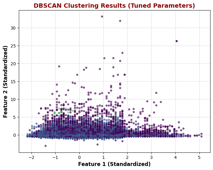
DBSCAN was applied to the dataset to identify density-based clusters and detect potential outliers. The algorithm was first run with its default parameters (eps=0.5, min_samples=5), leading to the formation of 78 clusters and 8408 outliers. This suggested that the dataset did not naturally form well-defined density-based clusters, and many points were classified as noise due to low local density.
Parameter Tuning for Better Clustering:
To improve the clustering results, eps was increased to 0.8 and min_samples was set to 10. With these adjusted parameters, DBSCAN identified 5 meaningful clusters while reducing the number of outliers to 3861. This adjustment helped DBSCAN recognize broader density-based structures instead of breaking the data into too many small, fragmented groups.
While parameter tuning improved DBSCAN's performance, the results still show significant overlap between clusters, making it less effective for structured segmentation. However, DBSCAN remains valuable for detecting outliers, which could represent unique customer behaviors or anomalies in the dataset. Compared to K-Means and Hierarchical Clustering, which provided clearer segmentations, DBSCAN is best suited for anomaly detection rather than structured clustering in this dataset.
Comparison of DBSCAN vs. Other Clustering Results
After testing K-Means,
Hierarchical Clustering, and
DBSCAN, the results highlight
significant differences in their performance and suitability for the dataset.
1. K-Means Clustering (Best Choice)
Identified 2 clusters, which align well with the dataset’s natural structure.
Achieved a high Silhouette Score, indicating well-separated clusters.
Fast and efficient, making it the most practical clustering method for this analysis.
2. Hierarchical Clustering (Supports K-Means)
Dendrogram suggested 2 primary clusters, reinforcing the K-Means findings.
More interpretable than DBSCAN but computationally expensive.
Useful for understanding cluster relationships, but less practical for large datasets.
3. DBSCAN (Not Ideal)
Initially detected 78 clusters and 8408 outliers — overly fragmented.
After tuning, detected only 1 main cluster with 1320 outliers, indicating poor segmentation.
More effective at detecting outliers than structured clusters.
RESULTS
K-Means was the best choice, as it provided the most clear and interpretable clusters.
Hierarchical Clustering confirmed the findings, making it useful for validation.
DBSCAN struggled, highlighting that it is better for datasets with non-uniform density or noise detection rather than well-separated groups.
Outlier detection using DBSCAN could still be useful for identifying anomalies or rare patterns in the dataset.
KEY TAKEAWAYS
K-Means should be used for final clustering because of its efficiency and strong separation.
DBSCAN can be useful for detecting anomalies, but not ideal for structured segmentation in this dataset.
Hierarchical Clustering provided valuable insights but is computationally expensive.
CONCLUSION
The clustering analysis helped uncover hidden patterns in customer behavior, providing valuable insights into how different groups interact. The data revealed that customers naturally fall into distinct segments, allowing for a better understanding of their preferences, financial habits, and engagement levels. This knowledge can be used to tailor services, improve customer experience, and create targeted marketing strategies.
Additionally, the analysis identified a group of customers with unusual behavior, which could indicate potential outliers or special cases that require a different approach. These could be customers with unique financial needs, irregular engagement patterns, or high-value clients who should be given personalized attention. By recognizing these patterns, businesses can enhance decision-making, optimize customer interactions, and better allocate resources to meet different needs.